
Scenarios 42 - 44
License

If you want to use the dataset or scripts on this page, please use the link below to generate the final list of papers that need to be cited.
Overview
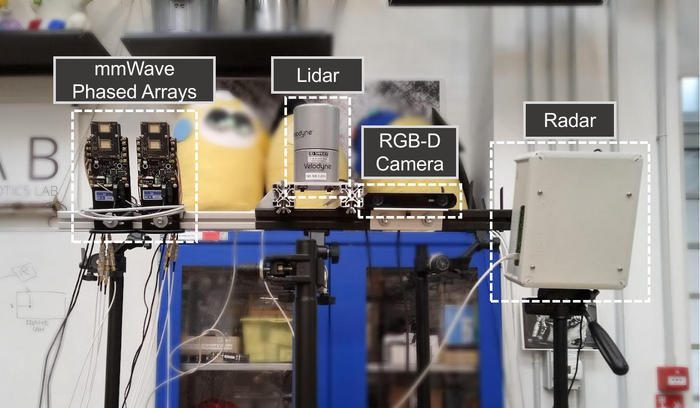
Illustration of the ISAC testbed utilized for data collection. Please refer to the detailed description of the testbed presented on the Data Collection page.
Scenarios 42 – 44 are collected in an indoor wireless environment. These scenarios are explicitly designed to compare the sensing capabilities of an ISAC communication system (with beamforming) with multi-modal sensing from a radar, lidar and RGB camera. These sceanrios have a single DeepSense unit, Unit1, comprised of four sensors: i) the ISAC subsystem (with one 60-GHz 16-element phased array for transmitting, one for receiving, and a baseband processing unit), ii) a 77 GHz radar, iii) a 2-cm resolution 3D LiDAR, and iv) a RGB-D camera. And this unit environment consists of a research laboratory in Politecnico di Milano. For more information on the testbed, refer to the detailed description in the Collected Data Section, or the testbed 7 description page.
The DeepSense ISAC 1 consists of three different scenarios, namely Scenarios 42, 43 and 44, each capturing data using different waveforms or faced with different sensing conditions. Scenarios 42 and 44 use a 1 GHz ISAC waveform where the OFDM communication signal occupies 95% of the total bandwidth, while in Scenario 43, the OFDM signal occupies only 10% of the total bandwidth. This allows … Furthermore, Scenarios 42 and 44 depict humans walking while Scenario 43 includes robots in the scene, which proved to be particularly reflective targets for the radar and ISAC sensing systems. Lastly, the the lidar and camera data provide interpretability and detection explanations for the ISAC and radar data. All the data is presented in the scenario videos below.
Collected Data
| Testbed | 7 |
|---|---|
| Total Samples | 6300 |
| Number of Samples | Scenario 42: 2100 || Scenario 43: 2100 || Scenario 44: 2100 |
| Number of Units | 2 |
| Data Modalities | RGB images, ISAC waveform, 3D LiDAR point-cloud, FMCW radar signal, |
| Unit1 | |
| Type | Static |
| Hardware Elements | Depth camera, 2x 60-GHz Phased Arrays, 3D LiDAR, FMCW radar |
| Data Modalities | RGB images, ISAC waveform, 3D LiDAR point-cloud, FMCW radar signal |
Sensors at Unit 1 (Static Communications and Sensing Unit)
- ISAC Sensor [Phased Array]: Consists of two 60-GHz mmWave Phased arrays and a baseband processing unit. Each phased array comprises of a rectangular uniform linear array (URA) panel with 16 elements, placed in 2 rows of 8 horizontal elements each. The phased arrays beamform according to the default codebook, which is an over-sampled DFT codebook of 64 beam directions. Out of the 64 codebook beams, only the beams 22 to 42 (21 beams in total) are used. These beams span roughly +- 30 degrees azimuth angle.
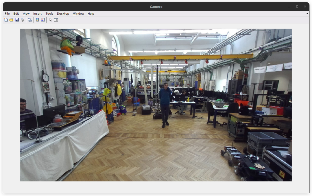
- Visual Sensor [Camera]: The main visual perception element in the testbed is the camera. This camera captures images at a resolution of 2208 x 1242 pixels and a frame rate of 30 FPS, which is aligned with the the beam sweeping rate of 10 Hz.
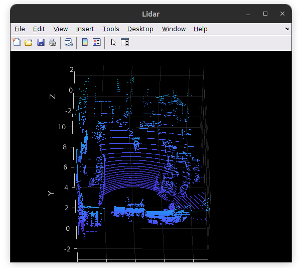
- 3D LiDAR Sensor: The LiDAR sensor in the testbed offers ranging and reflectivity data for objects within its field of view (approximately 10º above the horizontal to 30º below the horizontal). The lidar rotates at a frequency of 10Hz and captures 32 vertical channels simultaneously. Per rotation, it captures 2250 horizontal points sequentially. This results in 3D point cloud with ~1.3º vertical resolution and a ~0.16º horizontal resolution. The maximum range capability is 100 meters, with a typical resolution of 2 cm, allowing for comprehensive scanning and perception of the environment.
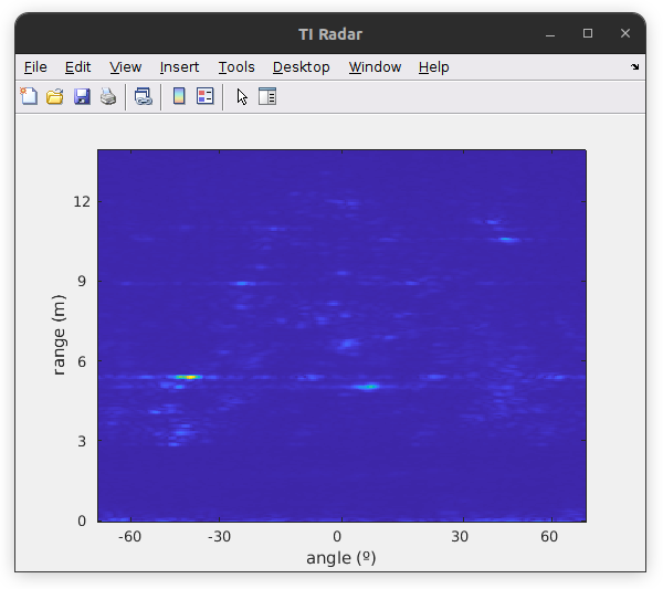
- FMCW radar: The testbed incorporates one Frequency-Modulated Continuous Wave (FMCW) radar sensor, which was configured with the parameters below. The data saved from the device is in the range-angle domain. For more information, see the Resources Section.
- Active TX antennas: 12
- Active RX antennas: 16
- # of samples per chirp: 256
- # of chirps per frame: 768
- ADC sampling rate: 8000 Ksps
- Chirp slope: 79 MHz/us
- Chirp Start Frequency: 77 GHz
- Ramp end time: 40 us
- ADC start time: 6 us
- Idle time: 5 us
- Receiver gain: 48 dB
- Radar frames per second: 10
Scenario Data Visualization
Download
Scenario 42-44 Download Links
How to Access Scenario Data?
Step 1. Download Scenario Data
1.1 – Log in above and click one of the download buttons to access the download page of each scenario.
1.2 – Select the modalities of interest and download (individually!) all zip files of the modality. For example, if you are interested in Scenario 42 isac and radar data, download the following files:
- scenario42.csv;
- scenario42_radar.zip001;
- scenario42_iq.zip.001, (…), scenario42_iq_zip.003
Step 2. Extract modality data
2.1 – Use the 7Zip utility to extract the ZIP files split into parts
2.2 – Select all zip files downloaded and 7Zip > Extract here.
(Objective: Each zip file has a scenario folder inside (e.g. “scenario42”) but a different modality. By extracting like this, the scenario folders will overlap and merge automatically, leading to a single scenario folder with the right structure. )
2.3 – Move the CSV file inside the extracted scenario folder.
If problems arise, see the Troubleshooting page.
Scenario 42 folder consists of two data sub-folders:
- unit1: Includes the data captured by unit 1
- resources: Includes scenario-specific information. In this case, the resources folder contains the transmitted ISAC waveform, a suggested colormap to display the ISAC sensing data and the radar axis which is required to visualize the radar data with a proper metric reference.
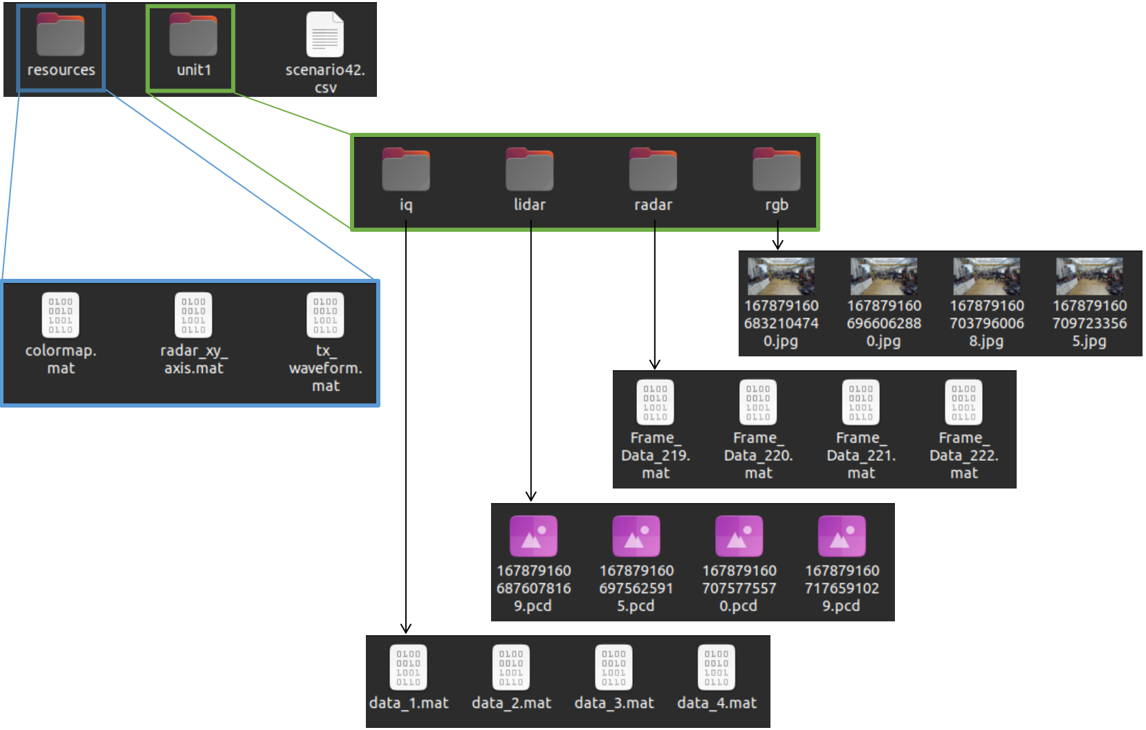
Besides data, the scenario folder includes one CSV file. This file “scenarioX.csv” file contains all samples. Each sample will have a timestamp, possibly sensor-specific metadata (like the beam used in the phased arrays), and paths to the data in each modality. This CSV helps loading all the data, as demonstrated in the MATLAB scripts at the end of this page.
Resources
What are the Additional Resources?
The additional resources in this scenario are three:
- tx_waveform.mat – The transmitted ISAC waveform. For communication purposes, the waveform can be used to demodulate the communication signal. For sensing purposes, as is the case in the example at the end of this page, the waveform is used to correlate and detect the received signal.
- colormap.mat – a suggested colormap to display the ISAC sensing data
- radar_xy_axis.mat – the radar axis that serves as a parameter and axis reference for the radar visualization
Additional Information: Explanation of Data in CSV
We further provide additional information for each sample present in the scenario dataset. The information provided here gives respect to the data listed in scenarioX.csv. Here we explain what each column means.
General information:
- Timestamp: This column represents the time of data capture in “hr-mins-secs.us” format with respect to the current timezone. It not only tells the time of the data collection but also tells the time difference between sample captures.
Sensor-specific information:
The sensors in these scenarios are rgb, lidar, radar, and iq. And sensors are associated with units. unit1_rgb1 refers to the first RGB camera of unit 1. unit2_gps1 refers to the first GPS of unit 2. If the unit only has one of that sensor type, the last number is not used, which is the case in these scenarios. Sensors may additionally have labels. For example, the sensor iq has three labels: iq_comm, iq_beam and iq_sweep. Labels are metadata acquired from that sensor. In these scenarios, only the iq sensor has metadata. The sensors and the labels are as follows:
-
unit1_rgb: the relative paths to the images collected by the camera.
-
unit1_lidar: the relative paths to the 3D pointclouds
- unit1_iq: the relative paths to the received ISAC waveforms. This sensor is called IQ because it contains the baseband received IQ data.
- unit1_iq_comm: Percentage of the signal bandwidth occupied by OFDM. The ISAC signal bandwidth is 1GHz, centered at 60 GHz. If the value in this column is 10, it means 10% of the bandwidth is occupied by OFDM (the case for Scenario 43). If the value is 95 it a wideband communication and sensing regime (Scenarios 42 and 44).
- unit1_iq_beam: As mentioned, the ISAC system uses phased arrays capable of analog beamforming. The system assumes 21 beams are used for communication purposes is a sequential way. This means that the sensing direction is constantly changing, according to the beam sweeping. Given a 0.1s sampling time, it takes 2.1 seconds to sweep all beams and sense the same direction again.
- unit1_iq_sweep: The index of the current beam sweep. Each sweep contains 21 samples, one for each beam.
- unit1_radar: the relative paths to the acquired data. Each radar sample is divided into two matrices, which are saved in a single .mat file. The matrices are: a) mag_data_static, corresponding to the range-angle data from the samples with zero speed (i.e., zero Doppler shift); and b) mag_data_dynamic, which contains the range-angle data for non-zero-Doppler samples.
An example table comprising of the first 10 rows of Scenario 42 is shown below.
| timestamp | unit1_iq | unit1_iq_comms_bandwidth | unit1_iq_sweep | unit1_iq_beam | unit1_radar | unit1_rgb | unit1_lidar |
|---|---|---|---|---|---|---|---|
| 12-00-06.900 | /unit1/iq/data_1.mat | 95 | 1 | 22 | /unit1/radar/Frame_Data_219.mat | /unit1/rgb/1678791606832104740.jpg | /unit1/lidar/1678791606876078169.pcd |
| 12-00-06.900 | /unit1/iq/data_2.mat | 95 | 1 | 23 | /unit1/radar/Frame_Data_219.mat | /unit1/rgb/1678791606966062880.jpg | /unit1/lidar/1678791606975625915.pcd |
| 12-00-07.000 | /unit1/iq/data_3.mat | 95 | 1 | 24 | /unit1/radar/Frame_Data_220.mat | /unit1/rgb/1678791607037960068.jpg | /unit1/lidar/1678791606975625915.pcd |
| 12-00-07.100 | /unit1/iq/data_4.mat | 95 | 1 | 25 | /unit1/radar/Frame_Data_221.mat | /unit1/rgb/1678791607097233565.jpg | /unit1/lidar/1678791607075775570.pcd |
| 12-00-07.200 | /unit1/iq/data_5.mat | 95 | 1 | 26 | /unit1/radar/Frame_Data_222.mat | /unit1/rgb/1678791607171497327.jpg | /unit1/lidar/1678791607176591029.pcd |
| 12-00-07.200 | /unit1/iq/data_6.mat | 95 | 1 | 27 | /unit1/radar/Frame_Data_222.mat | /unit1/rgb/1678791607229903425.jpg | /unit1/lidar/1678791607275349315.pcd |
| 12-00-07.300 | /unit1/iq/data_7.mat | 95 | 1 | 28 | /unit1/radar/Frame_Data_223.mat | /unit1/rgb/1678791607300323615.jpg | /unit1/lidar/1678791607275349315.pcd |
| 12-00-07.400 | /unit1/iq/data_8.mat | 95 | 1 | 29 | /unit1/radar/Frame_Data_224.mat | /unit1/rgb/1678791607369555893.jpg | /unit1/lidar/1678791607376691603.pcd |
| 12-00-07.500 | /unit1/iq/data_9.mat | 95 | 1 | 30 | /unit1/radar/Frame_Data_225.mat | /unit1/rgb/1678791607429359449.jpg | /unit1/lidar/1678791607476060062.pcd |
| 12-00-07.500 | /unit1/iq/data_10.mat | 95 | 1 | 31 | /unit1/radar/Frame_Data_225.mat | /unit1/rgb/1678791607501919472.jpg | /unit1/lidar/1678791607576494879.pcd |
Code Examples
Reproducing the ISAC Videos (MATLAB)
This script shows how to obtain the same plots shown in the videos. Consult the Tutorials Page for examples in Python and other applications of this data.
Part 1: Set Scenario Parameters and Read CSV
The first objective for visualizing the data is reading scenario data. In DeepSense, this is usually achieved by reading the DeepSense-format CSV file that comes with every scenario. First we define the scenario number to fetch the right csv file from the right folder. We load that file and see what columns it has. Note: this script assumes that this file is alongside a folder called “DeepSense Scenarios” which contains each scenario folder (e.g., “scenario42/”).
					scen_idx = 42;
folder = ['DeepSense Scenarios/scenario' num2str(scen_idx)];
csv_file = ['scenario' num2str(scen_idx) '.csv'];

% Read csv
fprintf("Reading: %s\n", csv_file);
csv_path = strcat(folder, filesep, csv_file);

opts = detectImportOptions(csv_path, 'Delimiter', ',');
opts.VariableTypes = repmat("string", 1, length(opts.VariableNames));
opts.DataLines = [1 inf];
opts.VariableNamesLine = 1;
dataframe = readmatrix(csv_path, opts);

% Print columns and rows information
fprintf(['Columns: [', repmat('''%s'' ', 1, length(opts.VariableNames)), ']\n'], ...
        dataframe(1,:))
n_rows = size(dataframe,1)-1;
fprintf('Number of Rows: %d\n', n_rows);
Reading: scenario42.csv
Columns: ['timestamp' 'unit1_iq' 'unit1_iq_comms_bandwidth' 'unit1_iq_sweep' 'unit1_iq_beam' 'unit1_radar' 'unit1_rgb' 'unit1_lidar']
Number of Rows: 2100
Part 2: Load Resources for Visualization
This section loads information from the radar data collection. These include the axis size, recommended color map and other parameters. It also initializes values required to plot the ISAC sensing signal.
					% Load Radar axis
load(strcat(folder, '/resources/radar_xy_axis.mat'), "x_axis", "y_axis")

% Load TX waveform for correlation
struct_waveform = struct2cell(load(strcat(folder, '/resources/tx_waveform.mat')));
tx_waveform = struct_waveform{1};

% Set small visualization variable
comms_bw = dataframe(2, dataframe(1,:)=="unit1_iq_comms_bandwidth");
if str2double(comms_bw) == 95; vis_e = 0.22; else; vis_e = 0.4; end

% Colormap
load(strcat(folder, '/resources/colormap.mat'), "map");
map=[zeros(100,3); map];

% ISAC sensing range and angle bins
range_res_sensing = 0.1464;
r=0:range_res_sensing/2:range_res_sensing*94;
angles = -54:5.4:54; %Sweep angles for comm
[R, PHI] = meshgrid(r,-angles);
Z = zeros(size(R));
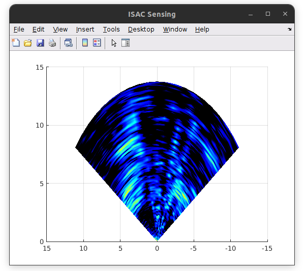
Part 3: Load Files and Visualize Data
To visualize all data, we must load all files first. To that end, we list all the files from reading the right columns in dataframe/csv file. Then we iterate over these files in the loop and select one by one and plot them. This script was designed to plot data as efficiently as possible, that is why the figures and axis are only created once (in the first iteration), and then only the data fields in the axes objects is changed.
					%% Load files and Plot

isac_files  = dataframe(2:end, dataframe(1,:)=="unit1_iq");
radar_files = dataframe(2:end, dataframe(1,:)=="unit1_radar");
rgb_files   = dataframe(2:end, dataframe(1,:)=="unit1_rgb");
lidar_files = dataframe(2:end, dataframe(1,:)=="unit1_lidar");

for i=1:n_rows
    fprintf("Row: %d | ", i);

    isac_file  = strcat(folder, isac_files(i));
    radar_file = strcat(folder, radar_files(i));
    rgb_file   = strcat(folder, rgb_files(i));
    lidar_file = strcat(folder, lidar_files(i));

    % Load Unit 1 - ISAC IQ
    load(isac_file, "waveform", "beam"); % import only iq

    % Load Unit 2 - Radar
    load(radar_file, "mag_data_static", "mag_data_dynamic");

    % Load Unit 3 - Image
    img = imread(rgb_file);

    % Load Unit 3 - Lidar Pointcloud
    ptCloud = pcread(lidar_file); % requires computer vision toolbox

    % Visualize Isac
    fprintf("Angle: %.1f\n", angles(beam - 21)); % 21 is the beam offset
    correlation = xcorr(waveform, tx_waveform); % correlate rx and tx signals
    [valR,idxR] = max(abs(correlation));
    snip = correlation(idxR-64:1:idxR+500);
    [pks, locs] = findpeaks(abs(snip));
    [~,idx_loc] = max(pks);
    % Z = zeros(size(R)); % uncomment this line for single scan visualization
    Z(beam - 21,:) = snip(locs(idx_loc):1:locs(idx_loc)+188);

    if i == 1
        figure('Name', 'ISAC Sensing', 'NumberTitle','off');
        s = surf(R.*cos(deg2rad(PHI)), R.*sin(deg2rad(PHI)), abs(Z).^vis_e);
        colormap(map);
        set(gcf,'color','w');
        s.EdgeColor = 'none';
        s.FaceColor = 'interp';
        view(-90,90);
        xlim([0 15]);
        ylim([-15 15]);
    else
        s.CData = abs(Z).^vis_e;
    end

    % Visualize Radar
    if i == 1
        figure('Name', 'TI Radar', 'NumberTitle','off');
        radar_ax = imagesc(mag_data_static' + mag_data_dynamic');
        a_tick = [18,65,129,193,240];
        a_axis = rad2deg(angle(x_axis(:,1)+y_axis(:,1)*1i));
        r_tick = 1:50:233;
        r_axis = sqrt(x_axis(33,:).^2+y_axis(33,:).^2);
        set(gca(), 'XTick', a_tick, 'XTickLabel', round(a_axis(a_tick)), ...
                   'YTick', r_tick, 'YTickLabel', round(r_axis(r_tick)), ...
                   'YDir', 'normal')
        xlabel("angle (º)");
        ylabel("range (m)");
    else
        radar_ax.CData = mag_data_static' + mag_data_dynamic';
    end

    % Visualize Image
    if i == 1
        figure('Name', 'Camera', 'NumberTitle','off');
        im_ax = imshow(img);
    else
        im_ax.CData = img;
    end

    % Visualize Lidar
    if i == 1
        player = pcplayer([-4,5],[-3,10],[-3,3], MarkerSize=2);

        set(player.Axes, "CameraPosition", [-27.2231 -393.3579 391.6075], ...
                         "CameraTarget", [1.9202 9.2605 -4.7717], ...
                         "CameraViewAngle", 1.2238, ...
                         "CameraUpVector", [-0.0026 0.6954 0.7186]);
        player.Axes.Parent.Name = 'Lidar';
        player.Axes.Parent.NumberTitle = 'off';
    end
    view(player, ptCloud);
    drawnow;
end
Acknowledgements
This dataset was build in collaboration with Davide Scazzoli, Simone Mentasti, Dario Tagliaferri and Marouan Mizmizi from the Politecnico di Milano, Italy.
License
If you want to use the dataset or scripts in this page, please cite the following two papers:
A. Alkhateeb, G. Charan, T. Osman, A. Hredzak, J. Morais, U. Demirhan, and N. Srinivas, “DeepSense 6G: A Large-Scale Real-World Multi-Modal Sensing and Communication Datasets,” available on arXiv, 2022. [Online]. Available: https://www.DeepSense6G.net
@Article{DeepSense,
author={Alkhateeb, Ahmed and Charan, Gouranga and Osman, Tawfik and Hredzak, Andrew and Morais, Joao and Demirhan, Umut and Srinivas, Nikhil},
title={DeepSense 6G: A Large-Scale Real-World Multi-Modal Sensing and Communication Dataset},
journal={IEEE Communications Magazine},
year={2023},
publisher={IEEE},}
D. Scazzoli, F. Linsalata, D. Tagliaferri, M. Mizmizi, D. Badini, M. Magarini, and U. Spagnolini, “Experimental Demonstration of ISAC Waveform Design Exploring Out-of-Band Emission,” IEEE International Conference on Communications Workshops (ICC Workshops), 2023
@INPROCEEDINGS{10283778,
author={Scazzoli, Davide and Linsalata, Francesco and Tagliaferri, Dario and Mizmizi, Marouan and Badini, Damiano and Magarini, Maurizio and Spagnolini, Umberto},
booktitle={2023 IEEE International Conference on Communications Workshops (ICC Workshops)},
title={Experimental Demonstration of ISAC Waveform Design Exploring Out-of-Band Emission},
year={2023},
pages={685-690},
doi={10.1109/ICCWorkshops57953.2023.10283778}}