Scenario 41
License
Overview

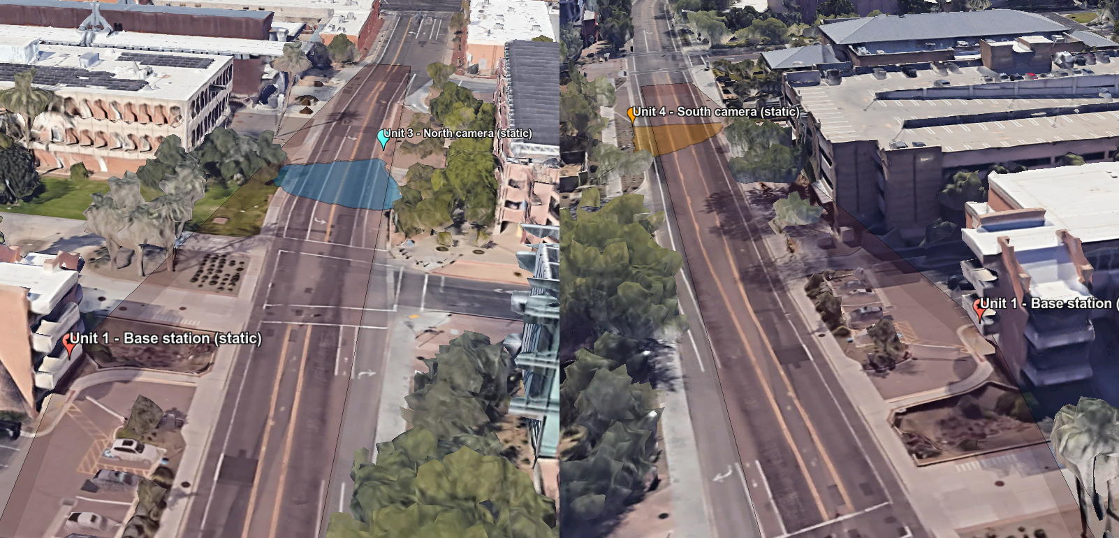
The data collection setup of Scenario 41. The top figure above shows the satellite view of the deployment, showing Unit 1 (base station) and Units 3 and 4, the distributed cameras. Units 1, 3, and 4 are static. The mobile unit, Unit 2 (car), passes in McAllister Avenue in both directions while communicating with the base station and being recorded by the distributed cameras.
The bottom figures show zoomed-in 3D views of the setup, showing the field-of-view of the cameras at the base station and roadside surveillance units. Units 3 and 4 are places at the ground level while Unit 1 is placed at a first floor height.
Scenario 41 is collected in an outdoor wireless environment explicitly designed to study distributed sensing at high-frequency V2I communication in the real world. The scenario utilizes DeepSense testbed 6 and two additional cameras. The collection setup consists of four units: (i) Unit 1, static receiver (base station) equipped with three 60-GHz mmWave Phased arrays facing -90, 0 and +90 degree directions, i.e., left, front, and, right, where the front face points at the street. Each phased array adopts a uniform linear array (ULA) with 16 elements and utilizes an over-sampled pre-defined codebook of 64 beam directions to receive the transmitted signal. It is further equipped with a 360-degree RGB camera to record the road. (ii) Unit 2, a mobile transmitter equipped with a 60-GHz quasi-omni antenna manually oriented towards the receiver unit, a GPS receiver to capture the real-time position information, and a wide view camera to provide information on its orientation and perspective. (iii) Units 3 and 4, static action cameras places in two locations along the road to emulate surveillance systems with distributed nodes.
S McAllister Avenue: It is a two-way street with 3 lanes (1 lane on each side with a passing lane in-between), a width of ~12 meters, and a vehicle speed limit of 30 mph (~48 kph). The avenue has several crosswalks and intersections, requiring diverse traffic patterns for the vehicles involved and several pedestrians. This avenue hosts a large variety of vehicles, such as buses, trucks, SUVs, and bikes, to name a few. In terms of wireless communication, the presence of big vehicles present the possibility of partial or complete user blockage. All these make the location diverse from the visual and wireless perspectives alike.
Collected Data
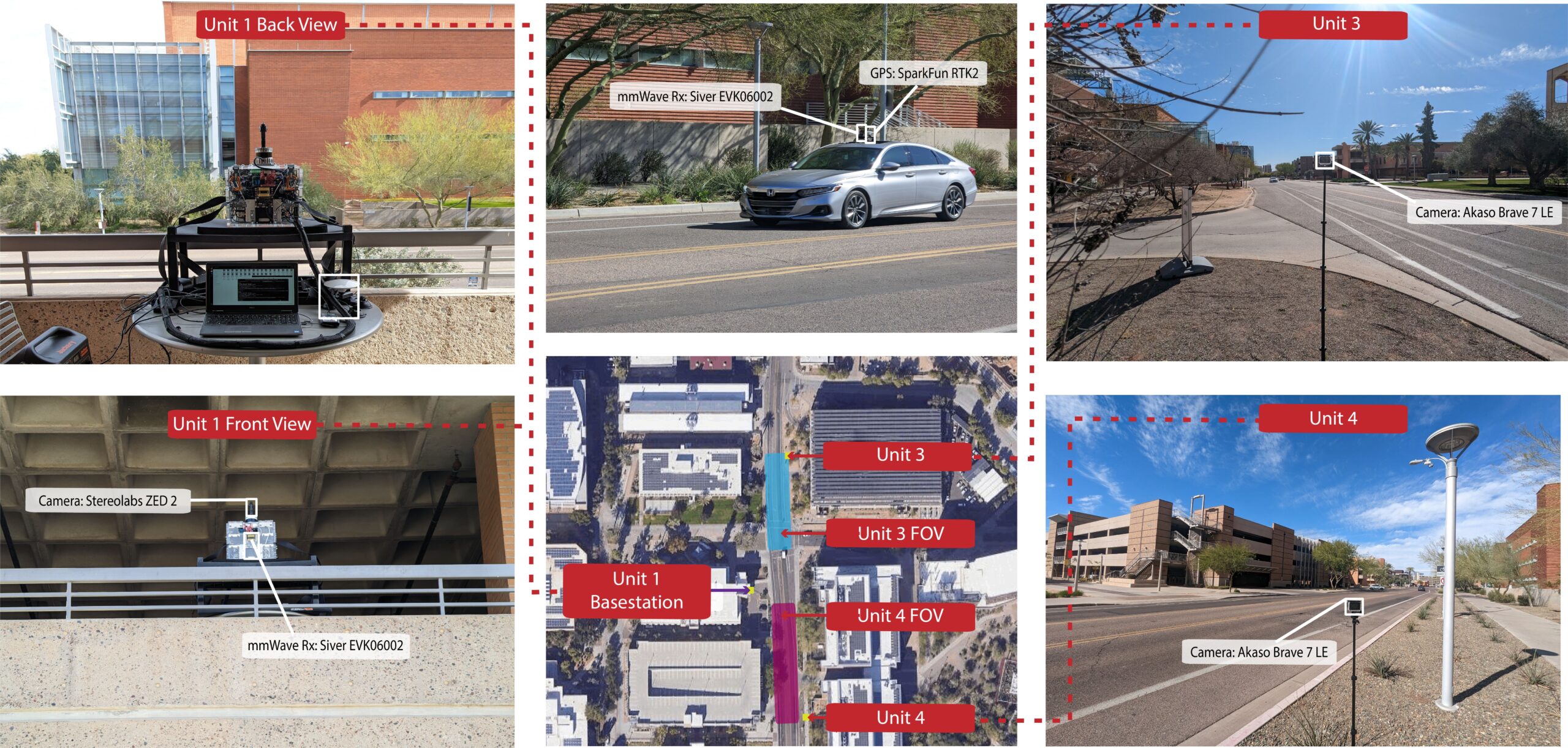
Sensors at Unit 1: (Static Receiver)
- Wireless Sensor [Phased Array]: Four 60-GHz mmWave Phased arrays facing four different directions, i.e., front, back, left, and right. Each phased array adopts a uniform linear array (ULA) with 16 elements and utilizes an over-sampled pre-defined codebook of 64 beam directions to receive the transmitted signal
- Visual Sensor [Camera]: The main visual perception element in the testbed is a 360-degree camera. This camera has the capability to capture 360-degree videos at a resolution of 5.7 K and a frame rate of 30 FPS. It is used to export one 180-degree view of the road.
Sensors at Unit 2: (Mobile Transmitter)
- Wireless Sensor [Phased Array]: A 60 GHz mmWave transmitter. The transmitter (Unit 2) continuously transmits using one antenna element of the phased array to realize near omnidirectional gain.
- Visual Sensor [Camera]: The ZED 2 camera is attached to the wireless sensor, allowing a user perspective of where the transmitter (unit 2) is focusing its power. This allows a great correlation of received power levels and transmitter orientation. This camera has a wide horizontal field-of-view (FoV) of 110 degrees and vertical FoV of 70 degrees. The images are captured from a single camera at a resolution of 1920 x 1080 pixels.
- Position Sensor [GPS Receiver]: To capture precise real-time locations for the unit 2 vehicle, a GPS-RTK receiver is employed. This receiver utilizes the L1 and L2 bands, enabling enhanced accuracy. As per the manufacturer’s specifications and the device’s horizontal dilution measures, the horizontal accuracies consistently remain within one meter of the true position.
Sensors at Unit 3 and Unit 4: (Static Cameras – North and South)
- Visual Sensor [Camera]: Units 3 and 4 are equipped with an action camera recording video at a resolution of 1920 x 1080 and a frame rate of 60 FPS. The frames are timestamped and then aligned with the remaining modalities, resulting in the selection of 10 frames per second to match the testbed capture rate.
| Testbed | 6 |
|---|---|
| Instances | 22500 |
| Number of Units | 4 |
| Data Modalities | RGB images, 64-dimensional received power vectors and GPS locations |
| Unit1 | |
| Type | Static |
| Hardware Elements | 360-degree RGB camera and 3 x mmWave phased array receiver |
| Data Modalities | 180-degree RGB images and 3 x 64-dimensional received power vector |
| Unit2 | |
| Type | Mobile |
| Hardware Elements | RGB-D camera, mmWave omni-directional transmitter, GPS receiver |
| Data Modalities | RGB images and GPS locations |
| Unit3 & Unit4 | |
| Type | Static |
| Hardware Elements | RGB camera |
| Data Modalities | RGB images |
Data Processing

Illustration of Testbed 6, the testbed utilized for data collection. In this case, Unit 1 is static.
Detailed description of the testbed presented here.
The DeepSense scenario creation pipeline involves two important stages: data processing and data visualization.
Data Processing: In the data processing stage, the collected sensor data is transformed into a common format that can be easily ingested and synchronized. This stage consists of two phases. Phase 1 focuses on converting data from different sensors into timestamped samples and organizing them in clear CSVs. It also involves interpolating GPS data to ensure proper synchronization. Phase 2 filters, organizes, and synchronizes the extracted data into a processed DeepSense scenario. This phase includes tasks such as data synchronization, filtering, sequencing, labeling, and data compression.
Data synchronization aligns samples from different sensors to a uniform sample rate based on timestamp proximity. Filtering involves rejecting samples based on specific criteria, including acquisition errors, non-coexistence of sensor sampling, and sequence filtering. Sequencing groups continuous samples together, ensuring a maximum 0.1-second gap between samples. Data labels provide additional contextual information, which can be derived from sensors or manually added. Data compression is performed to reduce file size, improve distribution efficiency, and allow selective downloading of specific modalities.
Data Visualization: The data visualization stage plays a crucial role in interpreting and understanding the dataset. It leverages the DeepSense Viewer library, providing a user interface (UI) for data visualization. Scenario videos are rendered, displaying all processed data synchronized over time. These videos facilitate navigation through the dataset, identification of relevant samples, and observation of propagation phenomena and sensor conditions.
Data Visualization
Download
How to Access Scenario Data?
Step 1. Download Scenario Data
1.1 – Click one of the Download buttons above to access the download page of each scenario.
1.2 – Select the modalities of interest and download (individually!) all zip files of the modality.
1.3 – Download the scenario csv (i.e. scenario41.csv), which indexes all data and is always needed.
Step 2. Extract modality data
2.1 – Install the 7Zip utility to extract ZIP files split into parts
2.2 – Select all zip files downloaded and select “Extract here”.
2.3 – Move the CSV file inside the scenario folder.
Scenario Folder Structure
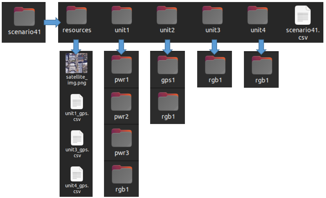
The DeepSense Scenario folder consists of the following sub-folders:
- unit1/unit2/unit3/unit4: Data captured by each unit
- resources: Scenario-specific annotations and other additional information. For more details, refer to the resources section below.
In case of problems during download or extraction, refer to the troubleshooting page.
Resources
What are the Additional Resources?
The additional resources in this scenario consist of:
- The static positions of units 1, 3, and 4. These are represented in text files with latitude and longitude coordinates.
- The top-view satellite image. This is the image presented as the background of the GPS plot in the video.
Additional Information: Explanation of Data in CSV
We further provide additional information for each sample present in the scenario dataset. The information provided here gives respect to the data listed in scenario41.csv. Here we explain what each column means.
General information:
- abs_index: Represents the sample absolute index. This is the sample index that is displayed in the video. This index remains unchanged from the sample collection all the way to the processed scenario. The advantage of absolute sample indices is the ability to perfectly backtrace information across processing phases and all the way to the raw collection data. If problems with the data exist, mentioning this sample index allows easier interaction with the DeepSense team. This also explains why the scenario starts at sample with index 1298 – the first 1297 samples were trimmed during scenario data preparation.
- Timestamp: This column represents the time of data capture in “hr-mins-secs.us” format with respect to the current timezone. It not only tells the time of the data collection but also tells the time difference between sample captures.
- seq_index: The index of a sequence. Samples have different sequence indices if there is a sufficiently large gap between data samples. Sequences denote data continuity. Consecutive samples are placed in the same sequence as long as the gap between them < 1/(2 * Fs), where Fs is our sampling frequency (10 Hz). This means that no consecutive pair of samples with a difference in timestamps larger than 0.2 seconds belongs to the same sequence.
Sensor-specific information:
Sensors can be gps1, pwr2, lidar1, radar3, etc. Sensors are associated with units. unit1_gps1 refers to the first GPS of unit 1. unit2_gps1 refers to the first GPS of unit 2. In these scenarios, only radar and power have more than one sensor per unit. It is important to recognize that for the power and radar sensors, the order (1, 2, 3, 4) is not arbitrary – it represents the directions they face. pwr1 regards the received power from the phased array in the front of the car. pwr2, pwr3, and pwr4 are from right, back, and left (clockwise direction), similarly with radar 1 to 4. Therefore, unit1_pwr1 will have information about the phased array in the front, and unit1_radar4 will have the raw radar samples from the radar pointing to the left. Sensors may additionally have labels. Labels are metadata acquired from that sensor. In these scenarios, only two sensors have metadata, and the labels are as follows:
- gps1_lat / gps1_lon / gps1_altitude: Latitude, longitude, and altitude.
- gps1_pdop / gps1_hdop / gps1_vdop: Position, horizontal and vertical, dilutions of precision. Measures of GPS confidence.
- pwr1_best-beam: a value between 0 and 63 representing the index of the beam that received the maximum power in the current time instant.
- pwr1_max-pwr / pwr1_min-pwr: values of the baseband received powers for a receive power vector of a certain array. These are the maximum and minimum powers computed in the baseband.
Beam indices in Unit 1 (Base Station)
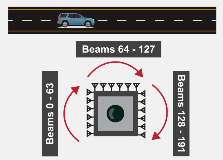
To better understand the beam indices in Unit 1 (base station), consider the figure to the right. This figure shows the collection setup of unit 1. Unit 1 is connected to 3 phased arrays (left: beams 0-63, front: beams 64-127, and right: beams 128-191). The front phased array is pointing at the road where unit 2 (a car equipped with a transmitter) passes in different lanes, with different speeds.
Note: To find the optimum receive/transmit beam in unit 1, the received powers across 192 beams need to be considered. Below we present a video showing how the optimum beam changes when unit 2 (the car) passes in front of unit 1.
Example video: Received power signatures across beams when unit 2 drives past the roadside unit 1
The video to the right shows a real-time visualization of the optimum beam as unit 2 passes in the street in front of unit 1. The plot displayed has 3 lines, one for each phased array. The x-axis is the index of the beam of the respective phased array. the y-axis is the received power by unit 1. We see that when the car is far to the left, the left phased array has an optimum beam close to the center. Then as the car drives through the base station the optimum beam passes to the center array and then to the right array.
An example table comprising the first 10 rows of data modalities, labels, and additional information.
| abs_index | timestamp | seq_index | unit1_rgb1 | unit1_pwr1 | unit1_pwr1_best-beam | unit1_pwr1_max-pwr | unit1_pwr1_min-pwr | unit1_pwr1_sweep-duration | unit1_pwr2 | unit1_pwr2_best-beam | unit1_pwr2_max-pwr | unit1_pwr2_min-pwr | unit1_pwr2_sweep-duration | unit1_pwr3 | unit1_pwr3_best-beam | unit1_pwr3_max-pwr | unit1_pwr3_min-pwr | unit1_pwr3_sweep-duration | unit2_gps1 | unit2_gps1_lat | unit2_gps1_lon | unit2_gps1_altitude | unit2_gps1_hdop | unit2_gps1_pdop | unit2_gps1_vdop | unit2_rgb1 | unit3_rgb1 | unit4_rgb1 | unit1_loc | unit3_loc | unit4_loc |
|---|---|---|---|---|---|---|---|---|---|---|---|---|---|---|---|---|---|---|---|---|---|---|---|---|---|---|---|---|---|---|---|
| 1298 | 14-02-53.363636 | 1 | unit1/rgb1/frame_14-02-53.920000.jpg | unit1/pwr1/pwr_14-02-47.372863.txt | 1 | 0.003686319 | 0.001038035 | 0.056344748 | unit1/pwr2/pwr_14-02-47.372863.txt | 20 | 0.001566936 | 0.001071432 | 0.056289196 | unit1/pwr3/pwr_14-02-47.372863.txt | 54 | 0.026089381 | 0.001063628 | 0.056298256 | unit2/gps1/gps_2578_14-02-53.363636.txt | 33.42052025 | -111.9289282 | 356.8744545 | 0.53 | 1.03 | 0.88 | unit2/rgb1/img_1753_14-02-46.257536.jpg | unit3/rgb1/frame_14-02-54.544164.jpg | unit4/rgb1/frame_14-02-54.810856.jpg | ../resources/static_pos_unit1.txt | ../resources/static_pos_unit3.txt | ../resources/static_pos_unit4.txt |
| 1299 | 14-02-53.454545 | 1 | unit1/rgb1/frame_14-02-54.000000.jpg | unit1/pwr1/pwr_14-02-47.472954.txt | 1 | 0.002955786 | 0.001044519 | 0.047629595 | unit1/pwr2/pwr_14-02-47.472954.txt | 21 | 0.001589676 | 0.001065635 | 0.04766798 | unit1/pwr3/pwr_14-02-47.472954.txt | 54 | 0.040937692 | 0.001078394 | 0.04771781 | unit2/gps1/gps_2579_14-02-53.454545.txt | 33.42052663 | -111.9289285 | 356.8698182 | 0.53 | 1.03 | 0.88 | unit2/rgb1/img_1756_14-02-46.381231.jpg | unit3/rgb1/frame_14-02-54.644166.jpg | unit4/rgb1/frame_14-02-54.910858.jpg | ../resources/static_pos_unit1.txt | ../resources/static_pos_unit3.txt | ../resources/static_pos_unit4.txt |
| 1300 | 14-02-53.545454 | 1 | unit1/rgb1/frame_14-02-54.080000.jpg | unit1/pwr1/pwr_14-02-47.572850.txt | 1 | 0.002810116 | 0.001065098 | 0.055731773 | unit1/pwr2/pwr_14-02-47.572850.txt | 37 | 0.001444921 | 0.001064793 | 0.055723429 | unit1/pwr3/pwr_14-02-47.572850.txt | 52 | 0.042558741 | 0.001097445 | 0.055736065 | unit2/gps1/gps_2580_14-02-53.545454.txt | 33.42053301 | -111.9289288 | 356.8651818 | 0.53 | 1.03 | 0.88 | unit2/rgb1/img_1758_14-02-46.461148.jpg | unit3/rgb1/frame_14-02-54.727501.jpg | unit4/rgb1/frame_14-02-54.994193.jpg | ../resources/static_pos_unit1.txt | ../resources/static_pos_unit3.txt | ../resources/static_pos_unit4.txt |
| 1301 | 14-02-53.636363 | 1 | unit1/rgb1/frame_14-02-54.200000.jpg | unit1/pwr1/pwr_14-02-47.673323.txt | 1 | 0.002454545 | 0.001031881 | 0.052060604 | unit1/pwr2/pwr_14-02-47.673323.txt | 22 | 0.001473646 | 0.001008901 | 0.052078247 | unit1/pwr3/pwr_14-02-47.673323.txt | 52 | 0.051304378 | 0.001081061 | 0.052082539 | unit2/gps1/gps_2581_14-02-53.636363.txt | 33.4205394 | -111.9289291 | 356.8605455 | 0.53 | 1.03 | 0.88 | unit2/rgb1/img_1760_14-02-46.547371.jpg | unit3/rgb1/frame_14-02-54.810836.jpg | unit4/rgb1/frame_14-02-55.094195.jpg | ../resources/static_pos_unit1.txt | ../resources/static_pos_unit3.txt | ../resources/static_pos_unit4.txt |
| 1302 | 14-02-53.727272 | 1 | unit1/rgb1/frame_14-02-54.280000.jpg | unit1/pwr1/pwr_14-02-47.772678.txt | 1 | 0.002992821 | 0.001073848 | 0.054139853 | unit1/pwr2/pwr_14-02-47.772678.txt | 24 | 0.001632266 | 0.001093172 | 0.054190397 | unit1/pwr3/pwr_14-02-47.772678.txt | 52 | 0.049569864 | 0.001112759 | 0.054175138 | unit2/gps1/gps_2582_14-02-53.727272.txt | 33.42054578 | -111.9289293 | 356.8559091 | 0.53 | 1.03 | 0.88 | unit2/rgb1/img_1762_14-02-46.629149.jpg | unit3/rgb1/frame_14-02-54.910838.jpg | unit4/rgb1/frame_14-02-55.177530.jpg | ../resources/static_pos_unit1.txt | ../resources/static_pos_unit3.txt | ../resources/static_pos_unit4.txt |
| 1303 | 14-02-53.818181 | 1 | unit1/rgb1/frame_14-02-54.360000.jpg | unit1/pwr1/pwr_14-02-47.772678.txt | 1 | 0.002992821 | 0.001073848 | 0.054139853 | unit1/pwr2/pwr_14-02-47.772678.txt | 24 | 0.001632266 | 0.001093172 | 0.054190397 | unit1/pwr3/pwr_14-02-47.772678.txt | 52 | 0.049569864 | 0.001112759 | 0.054175138 | unit2/gps1/gps_2583_14-02-53.818181.txt | 33.42055216 | -111.9289296 | 356.8512727 | 0.53 | 1.03 | 0.88 | unit2/rgb1/img_1764_14-02-46.713672.jpg | unit3/rgb1/frame_14-02-54.994173.jpg | unit4/rgb1/frame_14-02-55.277532.jpg | ../resources/static_pos_unit1.txt | ../resources/static_pos_unit3.txt | ../resources/static_pos_unit4.txt |
| 1304 | 14-02-53.909090 | 1 | unit1/rgb1/frame_14-02-54.440000.jpg | unit1/pwr1/pwr_14-02-47.872693.txt | 1 | 0.00316729 | 0.00102165 | 0.045477152 | unit1/pwr2/pwr_14-02-47.872693.txt | 25 | 0.001496372 | 0.001050649 | 0.04552412 | unit1/pwr3/pwr_14-02-47.872693.txt | 52 | 0.035709698 | 0.001076745 | 0.04553175 | unit2/gps1/gps_2584_14-02-53.909090.txt | 33.42055854 | -111.9289299 | 356.8466364 | 0.53 | 1.03 | 0.88 | unit2/rgb1/img_1766_14-02-46.798303.jpg | unit3/rgb1/frame_14-02-55.094175.jpg | unit4/rgb1/frame_14-02-55.360867.jpg | ../resources/static_pos_unit1.txt | ../resources/static_pos_unit3.txt | ../resources/static_pos_unit4.txt |
| 1305 | 14-02-54.000000 | 1 | unit1/rgb1/frame_14-02-54.560000.jpg | unit1/pwr1/pwr_14-02-47.973288.txt | 1 | 0.002007704 | 0.001076269 | 0.049135208 | unit1/pwr2/pwr_14-02-47.973288.txt | 22 | 0.001463468 | 0.001096266 | 0.049155951 | unit1/pwr3/pwr_14-02-47.973288.txt | 52 | 0.051372748 | 0.001095415 | 0.049129248 | unit2/gps1/gps_2585_14-02-54.000000.txt | 33.42056493 | -111.9289302 | 356.842 | 0.53 | 1.03 | 0.88 | unit2/rgb1/img_1769_14-02-46.925939.jpg | unit3/rgb1/frame_14-02-55.177510.jpg | unit4/rgb1/frame_14-02-55.460869.jpg | ../resources/static_pos_unit1.txt | ../resources/static_pos_unit3.txt | ../resources/static_pos_unit4.txt |
| 1306 | 14-02-54.090909 | 1 | unit1/rgb1/frame_14-02-54.640000.jpg | unit1/pwr1/pwr_14-02-48.072716.txt | 1 | 0.002038289 | 0.001060244 | 0.053576708 | unit1/pwr2/pwr_14-02-48.072716.txt | 24 | 0.001414347 | 0.001128209 | 0.053638935 | unit1/pwr3/pwr_14-02-48.072716.txt | 52 | 0.044910878 | 0.001095162 | 0.053628206 | unit2/gps1/gps_2586_14-02-54.090909.txt | 33.42057132 | -111.9289304 | 356.8409091 | 0.528181818 | 1.025454545 | 0.875454545 | unit2/rgb1/img_1771_14-02-47.011362.jpg | unit3/rgb1/frame_14-02-55.277512.jpg | unit4/rgb1/frame_14-02-55.544204.jpg | ../resources/static_pos_unit1.txt | ../resources/static_pos_unit3.txt | ../resources/static_pos_unit4.txt |

