Tutorials
About the Tutorials
Here you will find Python and MATLAB code to perform the essential data loading and visualization tasks on all modalities – Power, RGB images, GPS positions, Radar, and Lidar. Besides tasks on the main modality data, the group has acquired other relevant information (timestamp, number of connected satellites, etc. ) and performed annotations (sequence index, the direction of movement, object detection bounding boxes, etc.). The tutorials will also show how to access and leverage the metadata and annotations to visualize and understand propagation patterns.
We recommend watching the follow-along video to set up the DeepSense environment and run all tutorials.
If you have any related questions, please post them in Forum.
Table of Contents
Python
Setup Conda Environment
To execute the Python on this page, independently of your operative system, we suggest installing mamba (from github.com/conda-forge/miniforge#mambaforge) and setting up the environment via the prompt console. The console should appear (e.g., in the start menu) after the installation. Execute the following commands in the console to setup the environment:
					mamba create -n deepsense-env python=3.10
mamba activate deepsense-env
mamba install spyder numpy scikit-learn matplotlib pandas tqdm natsort
pip install open3d
Load & Display modalities [PWR | RGB | GPS | RADAR | 2D LIDAR]
First, we load all the scenario information, like the paths to each sample, which is present in the CSV.
					import os
import numpy as np
import pandas as pd
import matplotlib
import scipy.io as scipyio
import matplotlib.pyplot as plt

from tqdm import tqdm

# Absolute path of the folder containing the units' folders and scenarioX.csv
scenario_folder = r'C:\Users\WirelessIntelligence\Documents\DeepSense\Scenario9_Biodesign_2'

# Fetch scenario CSV
try:
    csv_file = [f for f in os.listdir(scenario_folder) if f.endswith('csv')][0]
    csv_path = os.path.join(scenario_folder, csv_file)
except:
    raise Exception(f'No csv file inside {scenario_folder}.')

# Load CSV to dataframe
dataframe = pd.read_csv(csv_path)
print(f'Columns: {dataframe.columns.values}')
print(f'Number of Rows: {dataframe.shape[0]}')
Columns: ['Unnamed: 0' 'index' 'unit1_rgb' 'unit1_pwr_60ghz' 'unit1_loc'
 'unit1_lidar' 'unit1_lidar_SCR' 'unit1_radar' 'unit2_loc' 'unit2_loc_cal']
Number of Rows: 5964
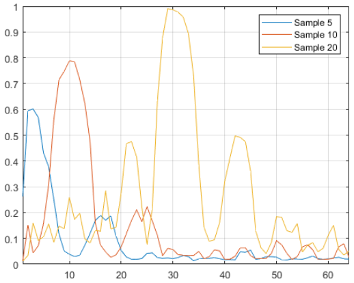
Then, we load each modality into memory and display the data. We start with the mmWave beam power measurements.
					N_BEAMS = 64
n_samples = 100
pwr_rel_paths = dataframe['unit1_pwr_60ghz'].values
pwrs_array = np.zeros((n_samples, N_BEAMS))

for sample_idx in tqdm(range(n_samples)):
    pwr_abs_path = os.path.join(scenario_folder,
                                pwr_rel_paths[sample_idx])
    pwrs_array[sample_idx] = np.loadtxt(pwr_abs_path)

# Select specific samples to display
selected_samples = [5, 10, 20]
beam_idxs = np.arange(N_BEAMS) + 1
plt.figure(figsize=(10,6))
plt.plot(beam_idxs, pwrs_array[selected_samples].T)
plt.legend([f'Sample {i}' for i in selected_samples])
plt.xlabel('Beam indices')
plt.ylabel('Power')
plt.grid()
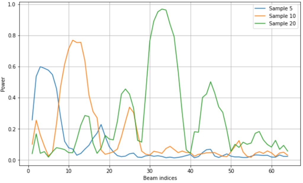
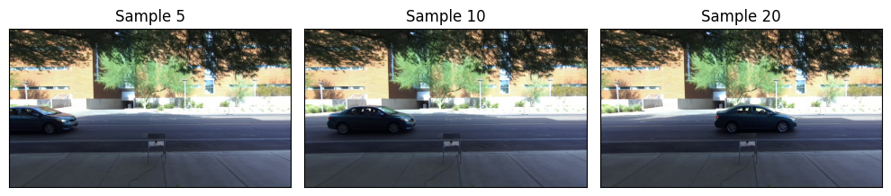
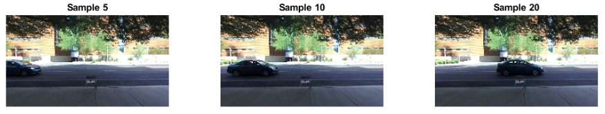
The images are a good modality to see next to understand the shapes of the power vectors. In scenario 9, ‘unit1_rgb’ refers to the camera. We load the images corresponding to the selected samples. We see that the car follows a general trend of moving from left to right, as does the peak of the main beam.
					img_rel_paths = dataframe['unit1_rgb'].values
fig, axs = plt.subplots(figsize=(10,4), ncols=len(selected_samples), tight_layout=True)
for i, sample_idx in enumerate(selected_samples):
    img_path = os.path.join(scenario_folder, img_rel_paths[sample_idx])
    img = plt.imread(img_path)
    axs[i].imshow(img)
    axs[i].set_title(f'Sample {sample_idx}')
    axs[i].get_xaxis().set_visible(False)
    axs[i].get_yaxis().set_visible(False)
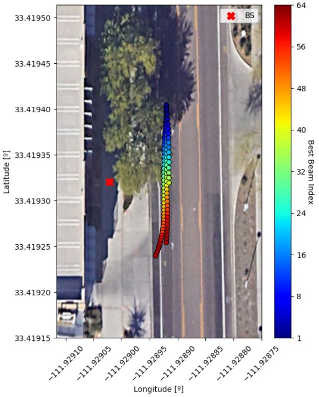
Next, GPS data. In scenario 9, ‘unit1_loc’ refers to the BS GPS position, and ‘unit2_loc’ or ‘unit2_loc_cal’ refers to UE positions. This information is detailed in each scenario page. We first load the necessary data.
					# BS position (take the first because it is static)
bs_pos_rel_path = dataframe['unit1_loc'].values[0]
bs_pos = np.loadtxt(os.path.join(scenario_folder,
                                 bs_pos_rel_path))
# UE positions
pos_rel_paths = dataframe['unit2_loc_cal'].values
pos_array = np.zeros((n_samples, 2)) # 2 = lat & lon

# Load each individual txt file
for sample_idx in range(n_samples):
    pos_abs_path = os.path.join(scenario_folder,
                                pos_rel_paths[sample_idx])
    pos_array[sample_idx] = np.loadtxt(pos_abs_path)

# Prepare plot: We plot on top of a Google Earth screenshot
gps_img = plt.imread('scen9_gps_img.png')

# Function to transform coordinates
def deg_to_dec(d, m, s, direction='N'):
    if direction in ['N', 'E']:
        mult = 1
    elif direction in ['S', 'W']:
        mult = -1
    else:
        raise Exception('Invalid direction.')

    return mult * (d + m/60 + s/3600)

# GPS coordinates from the bottom left and top right coordinates of the screenshot
gps_bottom_left, gps_top_right = ((deg_to_dec(33, 25, 8.94, 'N'),
                                   deg_to_dec(111, 55, 44.82, 'W')),
                                  (deg_to_dec(33, 25, 10.25, 'N'),
                                   deg_to_dec(111, 55, 43.50, 'W')))
Then we perform the GPS plot:
					# Important: screenshots taken with orientation towards North
best_beams = np.argmax(pwrs_array, axis=1)
fig, ax = plt.subplots(figsize=(6,8), dpi=100)
ax.imshow(gps_img, aspect='auto', zorder=0,
          extent=[gps_bottom_left[1], gps_top_right[1],
                  gps_bottom_left[0], gps_top_right[0]])

scat = ax.scatter(pos_array[:,1], pos_array[:,0], edgecolor='black', lw=0.7,
                  c=(best_beams / N_BEAMS), vmin=0, vmax=1,
                  cmap=matplotlib.colormaps['jet'])

cbar = plt.colorbar(scat)
cbar.set_ticks([0, 0.125, 0.25, 0.375, 0.5, 0.625, 0.75, 0.875, 1])
cbar.ax.set_yticklabels(['1', '8', '16', '24', '32', '40', '48', '56', '64'])
cbar.ax.set_ylabel('Best Beam Index', rotation=-90, labelpad=10)
ax.scatter(bs_pos[1], bs_pos[0], s=100, marker='X', color='red', label='BS')
ax.legend()
ax.ticklabel_format(useOffset=False, style='plain')
ax.tick_params(axis='x', labelrotation=45)
ax.set_xlabel('Longitude [º]')
ax.set_ylabel('Latitude [º]')

# We see about 2.5 car passes.
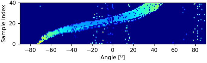
Next is Lidar 2D. In this case, we plot multiple samples across time to show a signature of the car’s movement.
					lidar_rel_paths =  dataframe['unit1_lidar_SCR'].values

# Compare noisy with denoised.
lidar_sample_size = 216

# Using the first 40 samples (almost the complete first car pass)
n_samp_first_seq = 40

# Append the lidar samples to array to show across a pass
lidar_frame = np.zeros((n_samp_first_seq, lidar_sample_size))
for sample_idx in range(n_samp_first_seq):
    lidar_file = os.path.join(scenario_folder, lidar_rel_paths[sample_idx])
    lidar_frame[sample_idx] = scipyio.loadmat(lidar_file)['data'][:,0]

angle_lims = [-90,90]
sample_lims = [0,n_samp_first_seq]
plt.figure(figsize=(6,2), dpi=120)
plt.imshow(np.fliplr(np.flipud(lidar_frame)),
           extent=[angle_lims[0], angle_lims[1], sample_lims[0], sample_lims[1]],
           aspect='equal')

plt.xlabel('Angle [º]')
plt.ylabel('Sample index')
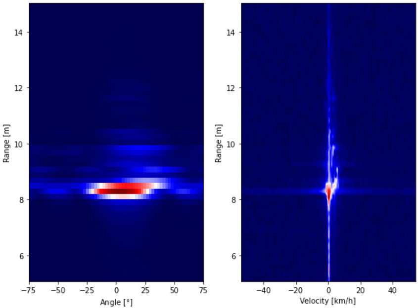
The last of the first set of plots is Radar. It requires the definition of a few more variables and functions, but it is also straightforward. Remember to see the video on the top of this page for more in-depth explanations.
					sample_idx = 20
radar_rel_paths = dataframe['unit1_radar'].values
radar_data = scipyio.loadmat(os.path.join(scenario_folder, radar_rel_paths[sample_idx]))['data']

RADAR_PARAMS = {'chirps':            128, # number of chirps per frame
                'tx':                  1, # transmitter antenna elements
                'rx':                  4, # receiver antenna elements
                'samples':           256, # number of samples per chirp
                'adc_sampling':      5e6, # Sampling rate [Hz]
                'chirp_slope': 15.015e12, # Ramp (freq. sweep) slope [Hz/s]
                'start_freq':       77e9, # [Hz]
                'idle_time':           5, # Pause between ramps [us]
                'ramp_end_time':      60} # Ramp duration [us]

samples_per_chirp = RADAR_PARAMS['samples']
n_chirps_per_frame = RADAR_PARAMS['chirps']
C = 3e8
chirp_period = (RADAR_PARAMS['ramp_end_time'] + RADAR_PARAMS['idle_time']) * 1e-6

RANGE_RES = ((C * RADAR_PARAMS['adc_sampling']) /
                    (2*RADAR_PARAMS['samples'] * RADAR_PARAMS['chirp_slope']))

VEL_RES_KMPH = 3.6 * C / (2 * RADAR_PARAMS['start_freq'] *
                          chirp_period * RADAR_PARAMS['chirps'])

min_range_to_plot = 5
max_range_to_plot = 15 # m
# set range variables
acquired_range = samples_per_chirp * RANGE_RES
first_range_sample = np.ceil(samples_per_chirp * min_range_to_plot /
                            acquired_range).astype(int)
last_range_sample = np.ceil(samples_per_chirp * max_range_to_plot /
                            acquired_range).astype(int)
round_min_range = first_range_sample / samples_per_chirp * acquired_range
round_max_range = last_range_sample / samples_per_chirp * acquired_range

# Range-Velocity Plot
vel = VEL_RES_KMPH * n_chirps_per_frame/2
ang_lim = 75 # comes from array dimensions and frequencies

def minmax(arr):
    return (arr - arr.min())/ (arr.max()-arr.min())

def range_velocity_map(data):
    data = np.fft.fft(data, axis=1) # Range FFT
    # data -= np.mean(data, 2, keepdims=True)
    data = np.fft.fft(data, axis=2) # Velocity FFT
    data = np.fft.fftshift(data, axes=2)
    data = np.abs(data).sum(axis = 0) # Sum over antennas
    data = np.log(1+data)
    return data

def range_angle_map(data, fft_size = 64):
    data = np.fft.fft(data, axis = 1) # Range FFT
    data -= np.mean(data, 2, keepdims=True)
    data = np.fft.fft(data, fft_size, axis = 0) # Angle FFT
    data = np.fft.fftshift(data, axes=0)
    data = np.abs(data).sum(axis = 2) # Sum over velocity
    return data.T

fig, axs = plt.subplots(figsize=(8,6), ncols=2, tight_layout=True)

# # Range-Angle Plot
radar_range_ang_data = range_angle_map(radar_data)[first_range_sample:last_range_sample]
axs[0].imshow(minmax(radar_range_ang_data), aspect='auto',
              extent=[-ang_lim, +ang_lim, round_min_range, round_max_range],
              cmap='seismic', origin='lower')
axs[0].set_xlabel('Angle [$\degree$]')
axs[0].set_ylabel('Range [m]')


radar_range_vel_data = range_velocity_map(radar_data)[first_range_sample:last_range_sample]
axs[1].imshow(minmax(radar_range_vel_data), aspect='auto',
              extent=[-vel, +vel, round_min_range, round_max_range],
              cmap='seismic', origin='lower')
axs[1].set_xlabel('Velocity [km/h]')
axs[1].set_ylabel('Range [m]')
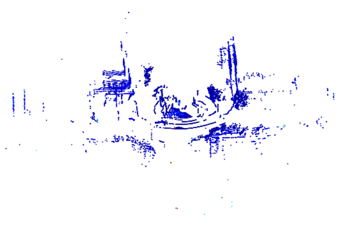
Display 3D Lidar Point Cloud [Static mode]
We use Open3D to visualize the 3D point cloud from the Lidar one frame at a time. Note that the 3D Lidar files are .ply or .csv files, while 2D Lidar files are .mat files. This static method is meant to work with .ply files, but the Dynamic method (see next) works with both .ply and .csv files.
					import open3d as o3d
import os
import matplotlib.pyplot as plt
from natsort import natsorted
import numpy as np

# Path to lidar (pointcould) files
path = r"C:\Users\UserName\DeepSense\Scenario31\unit1\lidar_data"
address = natsorted(os.listdir(path))
outpath = '.'
vis = o3d.visualization.Visualizer()

vis.create_window(visible=True)
vis.poll_events()
vis.update_renderer()
cloud = o3d.io.read_point_cloud(path+"/"+ address[0])
vis.add_geometry(cloud)

# (optional) In case a certain view is desired for the matplotlib shots:
params = {
    "field_of_view" : 60.0,
    "front" : [ -0.01093, 0.0308, 0.9994 ],
    "lookat" : [ -18.9122, -18.4687, 7.3131],
    "up" : [ 0.5496, 0.8351, -0.0197 ],
    "zoom" : 0.3200
    } # These parameters can be copied directly from the visualizer by doing Ctrl+C

opt = vis.get_render_option()
o3d.visualization.ViewControl.set_zoom(vis.get_view_control(), params['zoom'])
o3d.visualization.ViewControl.set_lookat(vis.get_view_control(), params['lookat'])
o3d.visualization.ViewControl.set_front(vis.get_view_control(),params['front'])
o3d.visualization.ViewControl.set_up(vis.get_view_control(), params['up'])
					for i in range(1): # number of frames to load
    cloud.points = o3d.io.read_point_cloud(path+"/"+ address[i]).points
    print(path+"/"+ address[i])
    vis.update_geometry(cloud)
    vis.poll_events()
    vis.update_renderer()

    ## Plot with matplotlib
    color = np.asarray(vis.capture_screen_float_buffer(True))
    plt.imshow(color)
    plt.title(f'Sample {i+1}')
    plt.savefig(outpath+"/"+ address[i].split('.')[0] + '.png', dpi=300)
    plt.tight_layout()
    plt.pause(0.1)
vis.destroy_window()
[Open3D INFO] WebRTC GUI backend enabled.
C:\Users\UserName\DeepSense\Scenario31\unit1
\lidar_data/Frame_1175_01_29_49_587.ply
Display 3D Lidar Pointcloud [Dynamic mode]
For the dynamic visualization, most of the setup is the same, but it outputs an interactive visualization that allows us to analyze the data with more flexibility.
					import os
import numpy as np
import pandas as pd
import open3d as o3d
from natsort import natsorted
import matplotlib
import matplotlib.pyplot as plt

colormap = matplotlib.colormaps['jet']

# Path to lidar (pointcould) files
source_folder = r"G:/DeepSense-scenarios/scenario34/unit1/lidar_data"
relative_paths = natsorted(os.listdir(source_folder))
csv_format = relative_paths[0].endswith('csv')
load_files = [source_folder + "/" + path for path in relative_paths]
save_frames = False

vis = o3d.visualization.Visualizer()

vis.create_window(width=600, height=600)
vis.poll_events()
vis.update_renderer()
opt = vis.get_render_option()
opt.point_size = 2
opt.background_color = np.asarray([0, 0, 0])
opt.save_to_json('params.json')

view_ctr = vis.get_view_control()

# (optional) In case a certain view is desired for the matplotlib shots:
# These parameters can be copied directly from the visualizer by doing Ctrl+C
params = {
    "field_of_view" : 60.0,
    "front" : [ 0.89933620757791011, -0.02479685035379222, 0.43655412259182019 ],
    "lookat" : [ 5.4501878245913096, -2.4011275125017444, 2.2753175793425693 ],
    "up" : [ -0.4371391667163444, -0.027731978813576672, 0.89896623199852355 ],
    "zoom" : 0.06
    }

# Column to display in case the Lidar file is in CSV format
col = [' RANGE (mm)', ' SIGNAL', ' REFLECTIVITY', ' NEAR_IR'][0]

percentile = 95 # for normalization
if csv_format:
    df = pd.read_csv(load_files[0])
    norm_factor = np.percentile(np.array(df[col].values), percentile)
else:
    points = np.asarray(o3d.io.read_point_cloud(load_files[0]).points)
    norm_factor = np.percentile(np.linalg.norm(points, axis=1), percentile)

cloud = o3d.geometry.PointCloud()

idxs = np.arange(len(load_files))
for i in idxs:

    if csv_format:
        df = pd.read_csv(load_files[i])
        xyz = np.stack((df[' X (mm)'].values, df[' Y (mm)'].values, df[' Z (mm)'].values)).T
        cloud.points = o3d.utility.Vector3dVector(xyz)
        arr = np.array(df[col].values)
        # colors  Type: | float64 array of shape (num_points, 3), range [0, 1] , use numpy.asarray() to access
        cloud.colors = o3d.utility.Vector3dVector(colormap(arr/norm_factor)[:,:3]) #:3 to remove the alpha
    else:
        cloud.points = o3d.io.read_point_cloud(load_files[i]).points
        distances = np.linalg.norm(np.asarray(cloud.points), axis=1)
        cloud.colors = o3d.utility.Vector3dVector(colormap(distances/norm_factor)[:,:3])

    if i == idxs[0]:
        vis.add_geometry(cloud)
        # Uncomment below to apply the parameters
        # Note: might make the data if wrongly set
        view_ctr.change_field_of_view(params['field_of_view'])
        view_ctr.set_zoom(params['zoom'])
        view_ctr.set_lookat(params['lookat'])
        view_ctr.set_front(params['front'])
        view_ctr.set_up(params['up'])

    print(load_files[i])
    vis.update_geometry(cloud)
    vis.poll_events()
    vis.update_renderer()

    if save_frames:
        color = vis.capture_screen_float_buffer(True)
        color_array = np.asarray(color)
        plt.imshow(color_array)
        sample_text = f'Sample {i+1}'
        plt.title(sample_text)
        plt.savefig(sample_text + '.png', dpi=300)
        plt.tight_layout()

vis.destroy_window()
Jupyter environment detected. Enabling Open3D WebVisualizer.
[Open3D INFO] WebRTC GUI backend enabled.
[Open3D INFO] WebRTCWindowSystem: HTTP handshake server disabled.
G:/DeepSense-scenarios/scenario34/unit1/lidar_data/lidar_data_154.ply
G:/DeepSense-scenarios/scenario34/unit1/lidar_data/lidar_data_155.ply
G:/DeepSense-scenarios/scenario34/unit1/lidar_data/lidar_data_156.ply
G:/DeepSense-scenarios/scenario34/unit1/lidar_data/lidar_data_157.ply
G:/DeepSense-scenarios/scenario34/unit1/lidar_data/lidar_data_158.ply
G:/DeepSense-scenarios/scenario34/unit1/lidar_data/lidar_data_159.ply
G:/DeepSense-scenarios/scenario34/unit1/lidar_data/lidar_data_160.ply
...
(And we obtain visualizations like the video below)
Matlab
Load modalities [PWR | RGB | GPS | RADAR | 2D LIDAR]
As done in Python, we first load the modality data into memory.
					% Inputs:
scen_path = "C:\Users\Morais\Documents\PHD\Work\DeepSense\DeepSense[95%]\Scenario9_Biodesign_2";
csv_file = "scenario9.csv";
n_samples = 100;
first_sample = 1;
unit = 1;
modalities = {'pwr_60ghz', 'loc', 'rgb', 'radar', 'lidar'};

% [Scenario 9]
% Available units: 1, 2
% Available modalities: 'pwr_60ghz', 'loc', 'rgb', 'radar', 'lidar'

% Set constants
UNIT_STR = "unit" + int2str(unit) + "_";
SAMPLE_DIMENSIONS.loc = [2, 1];
SAMPLE_DIMENSIONS.pwr_60ghz = [64, 1];
SAMPLE_DIMENSIONS.rgb = [540, 960, 3];
SAMPLE_DIMENSIONS.lidar = [460, 2];
SAMPLE_DIMENSIONS.radar = [4, 256, 128];

% Read csv
fprintf("Reading: %s\n", csv_file);
csv_path = strcat(scen_path, filesep, csv_file);

opts = detectImportOptions(csv_path, 'Delimiter', ',');
opts.VariableTypes = repmat("string", 1, length(opts.VariableNames));
opts.DataLines = [1 inf];
opts.VariableNamesLine = 1;
dataframe = readmatrix(csv_path, opts);

% Print columns and rows information
fprintf(['Columns: [', repmat('''%s'' ', 1, length(opts.VariableNames)), ']\n'], ...
        dataframe(1,:))
n_rows = size(dataframe,1)-1;
fprintf('Number of Rows: %d\n', n_rows);

% Define the range of samples to load
last_sample = first_sample + n_samples - 1;
sample_range = first_sample:last_sample;

% Load data from each file
fprintf('Reading %d samples... \n', n_samples);
data = {};
for k=1:length(modalities)
    mod = modalities{k};
    data.(mod) = zeros([n_samples,SAMPLE_DIMENSIONS.(mod)]);
    files = dataframe(2:end,dataframe(1,:)==(UNIT_STR + mod));
    for ii=sample_range
        % Get the path from the CSV
        try
            temp = regexp(files{ii}, '/', 'split');
            file_parts = temp(2:end);
        catch
            fprintf("Path is improperly formated. Rectify CSV.\n");
        end

        % Put together the file parts to form the full absolute path
        file_path_parts = scen_path;
        for jj=1:length(file_parts)
            file_path_parts = [file_path_parts filesep file_parts{jj}]; %#ok<AGROW>
        end
        file_path = join(file_path_parts, '');

        % Loading methods for specific modalities
        new_idx = find(sample_range == ii);
        if any(mod == ["loc", "loc_cal", "pwr_60ghz"])
            fid = fopen(file_path, 'r');
            data.(mod)(new_idx,:) = cell2mat(textscan(fid, '%f'));
            fclose(fid);
        end

        if mod == "rgb"
            img = imread(file_path);
            data.(mod)(new_idx,:,:,:) = imread(file_path);
        end

        if mod == "lidar"
            data.(mod)(new_idx,:,:) = load(file_path).data;
        end

        if mod == "radar"
            data.(mod)(new_idx,:,:,:) = load(file_path).data;
        end
    end
end

disp('Done!')
disp(data);
Reading: scenario9.csv
Columns: ['index' 'unit1_rgb' 'unit1_pwr_60ghz' 'unit1_loc' 'unit1_lidar' 'unit1_lidar_SCR' 'unit1_radar' 'unit2_loc' 'unit2_loc_cal' ]
Number of Rows: 5964
Reading 100 samples...
Done!
    pwr_60ghz: [100×64 double]
          loc: [100×2 double]
          rgb: [100×540×960×3 double]
        radar: [100×4×256×128 double]
        lidar: [100×460×2 double]
Display PWR & RGB
After loading the data and understanding its structure, one can display it in any way. We show examples of the mmWave beam power measurements and RGB images. Although GPS, Radar, and 2D lidar are omitted, we expect these visualizations to be a programming language translation from the Python code above. If you’d find it useful to have explicit examples of how to do this, let us know via email in the Forum.
					% Plot power
selected_samples = [5, 10, 20];

figure()
plot(1:64, data.pwr_60ghz(selected_samples, :))
legend({'Sample 5', 'Sample 10', 'Sample 20'})
xlim([1,64])
grid()

% Plot RGB Img
figure('Position', [20 240 1240 280])
for i=1:3
    subplot(1,3,i)
    imshow(cast(squeeze(data.rgb(selected_samples(i),:,:,:)), 'uint8'))
    title(strcat("Sample ", string(selected_samples(i))))
end
Display 3D Lidar Pointcloud
Lastly, the visualization of a 3D lidar point cloud in Matlab. This way is one of the simplest, but it is likely that there are better tools to display and analyze this data in Matlab.
					path="C:\Users\UserName\DeepSense\Scenario31\unit1\lidar_data"; % path to .ply file
path_req="."; % path to save directory
file = fullfile(path, '*.ply');
theFiles = dir(file);

for k = 1 : length(theFiles)
    baseFileName = theFiles(k).name;
    fullFileName = fullfile(theFiles(k).folder, baseFileName);
    ptCloud(k) = pcread(fullFileName);
    %figure('units','normalized','outerposition',[0 0 1 1])
    pcshow(ptCloud(k));
    zoom(3)
    axis off
    savefig(path_req+"/"+baseFileName+".fig")
    close
end